第11章 时间序列 时间序列数据的意义取决于具体的应⽤场景,主要有以下⼏种:
时间戳(timestamp),特定的时刻。
固定时期(period),如2007年1⽉或2010年全年。
时间间隔(interval),由起始和结束时间戳表示。时期
实验或过程时间,每个时间点都是相对于特定起始时间的⼀个度量。例如,从放⼊烤箱时起,每秒钟饼⼲的直径。
11.1 日期和时间数据类型及⼯具 Python时间日期相关的常用标准库:
11.1 ⽇期和时间数据类型及⼯具 1 2 3 4 5 6 7 8 9 10 11 12 13 14 15 16 17 18 19 20 21 22 23 24 25 26 27 28 29 30 31 32 from datetime import datetime,timedeltanow = datetime.now() print (now)print (now.year, now.month, now.day)print (now.hour, now.min , now.second)delta = datetime(2011 , 1 , 7 ) - datetime(2008 , 6 , 24 , 8 , 15 ) print (delta)print (delta.days)print (delta.seconds)start = datetime(2011 , 1 , 7 ) print (start + timedelta(12 ))print (start - 2 * timedelta(12 ))
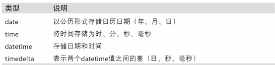
datetime模块中的数据类型
字符串和datetime的相互转换
利⽤str或strftime⽅法(传⼊⼀个格式化字符串),datetime对象和pandas的Timestamp对象可以被格式化为字符串:
1 2 3 4 5 6 7 8 9 10 11 12 13 14 15 16 17 18 19 20 21 22 from datetime import datetime,timedeltastamp = datetime(2011 , 1 , 3 ) print (str (stamp))print (stamp.strftime('%Y-%m-%d' ))value = '2011-01-03' print (datetime.strptime(value, '%Y-%m-%d' ))datestrs = ['7/6/2011' , '8/6/2011' ] print ([datetime.strptime(x, '%m/%d/%Y' ) for x in datestrs])
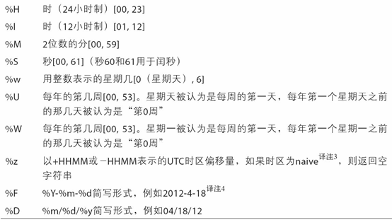
datetime格式化编码。
datetime.strptime通过将字符串对象转为datetime对象,但是每次都要编写格式定义是很麻烦的事情,这时候就可以使用from dateutil.parser import parse.dateutil可以解析几乎所有人类能够理解的日期表示形式 :
1 2 3 4 5 6 7 8 9 10 11 12 13 from dateutil.parser import parseprint (parse('2011-01-03' ))print (parse('Jan 31, 1997 10:45 PM' ))print (parse('6/12/2011' , dayfirst=True ))
pandas使用to_datetime方法解析多种不同的日期表示形式.
1 2 3 4 5 6 7 8 9 10 11 12 13 14 15 16 17 18 19 20 import pandas as pddatestrs = ['2011-07-06 12:00:00' , '2011-08-06 00:00:00' ] print (pd.to_datetime(datestrs))idx = pd.to_datetime(datestrs + [None ]) print (idx)print (idx[2 ])print (pd.isnull(idx))
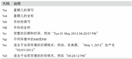
特定于当前环境的⽇期格式
11.2 时间序列基础 知识预备:
1 2 3 4 5 6 7 8 9 10 11 12 13 14 15 16 17 18 19 20 21 22 23 24 25 26 27 28 29 30 31 32 33 34 35 36 37 38 39 40 41 import numpy as npimport pandas as pdx = pd.Series(np.arange(10 )) print (x)y = pd.Series(np.arange(10 )) print (y[::2 ])print (x + y[::2 ])
pandas最基本的时间序列类型就是以时间戳Datetime为索引的Series.
以Datetime为index的类型是DatetimeIndex
pandas⽤NumPy的datetime64数据类型以纳秒形式存储==时间戳==
DatetimeIndex中的各个标量值是pandas的Timestamp 对象DatetimeIndex的元素是时间戳
TimeStamp 可以随时⾃动转换为datetime 对象。此外,它还可以存储频率信息(如果有的话),且知道如何执⾏时区转换以及其他操作
1 2 3 4 5 6 7 8 9 10 11 12 13 14 15 16 17 18 19 20 21 22 23 24 25 26 27 28 29 30 31 32 33 34 35 36 37 38 39 40 41 42 43 44 45 46 47 48 49 50 51 52 53 54 55 56 57 58 from datetime import datetimeimport numpy as npimport pandas as pdnp.random.seed(888 ) dates = [datetime(2011 , 1 , 2 ), datetime(2011 , 1 , 5 ), datetime(2011 , 1 , 7 ), datetime(2011 , 1 , 8 ), datetime(2011 , 1 , 10 ), datetime(2011 , 1 , 12 )] ts = pd.Series(np.random.randn(6 ), index=dates) print (ts)print (ts.index)print (ts[::2 ])print (ts + ts[::2 ])print (ts.index.dtype)print (type (ts.index[0 ]))print (ts.index[0 ])
索引、选取、子集构造
DatetimeIndex索引有一种专属索引方法:
传⼊⼀个可以被解释为日期的字符串
甚至只传入不部分字符串(如传入“年”或“年⽉”)就可以索引得到
传入Datatime对象
使用不存在于该时间序列中的时间戳 对其进⾏切⽚(即范围查询)
使用truncate方法
注意,以上五种方法产⽣的都是源时间序列的视图 ,这意味着,没有数据被复制,对切⽚进⾏修改会反映到原始数据上。
1 2 3 4 5 6 7 8 9 10 11 12 13 14 15 16 17 18 19 20 21 22 23 24 25 26 27 28 29 30 31 32 33 34 35 36 37 38 39 40 41 42 43 44 45 46 47 48 49 50 51 52 53 54 55 56 57 58 59 60 61 62 63 64 65 66 67 68 69 70 71 72 73 74 75 76 77 78 79 80 81 82 83 84 85 86 87 88 89 90 91 92 93 94 95 96 97 98 99 100 101 102 103 104 105 106 107 108 109 from datetime import datetimeimport numpy as npimport pandas as pdnp.random.seed(888 ) dates = [datetime(2011 , 1 , 2 ), datetime(2011 , 1 , 5 ), datetime(2011 , 1 , 7 ), datetime(2011 , 1 , 8 ), datetime(2011 , 1 , 10 ), datetime(2011 , 1 , 12 )] ts = pd.Series(np.random.randn(6 ), index=dates) print (ts)stamp = ts.index[2 ] print (stamp)print (ts[stamp])print (ts['1/10/2011' ])print (ts['20110110' ])longer_ts = pd.Series(np.random.randn(1000 ), index=pd.date_range('1/1/2000' , periods=1000 )) print (longer_ts)print (longer_ts['2001' ])print (longer_ts['2001-05' ])print (ts[datetime(2011 , 1 , 7 ):])print (ts)print (ts['1/6/2011' :'1/11/2011' ])print (ts.truncate(after='1/9/2011' ))
带有重复索引的时间序列
1 2 3 4 5 6 7 8 9 10 11 12 13 14 15 16 17 18 19 20 21 22 23 24 25 26 27 28 29 30 31 32 33 34 35 36 37 38 39 40 41 42 43 44 45 46 47 import numpy as npimport pandas as pddates = pd.DatetimeIndex(['1/1/2000' , '1/2/2000' , '1/2/2000' , '1/2/2000' , '1/3/2000' ]) dup_ts = pd.Series(np.arange(5 ), index=dates) print (dup_ts)print (dup_ts.index.is_unique)print (dup_ts['1/3/2000' ])print (dup_ts['1/2/2000' ])grouped = dup_ts.groupby(level=0 ) print (grouped.mean())print (grouped.count())
11.3 日期的范围、频率以及移动 部分基本的时间序列频率(freq参数)
别名
偏移量类型
说明
D
Day
每日历日
B
BusinessDay
每工作日
H
Hour
每小时
T或min
Minute
每分
S
Second
每秒
L或ms
Milli
每毫秒
U
Micro
每微秒
M
MonthEnd
每月最后一个日历日
BM
BusinessMonthEnd
每月最后一个工作日
MS
MonthBegin
每月第一个日历日
BMS
BusinessMonthBegin
每月第一个工作日
W-MON
Week
从指定的星球几开始算起,每周
WOM-1MON
WeekOfMonth
每月第一,第二…个星期几
1 2 3 4 5 6 7 8 9 10 11 12 13 14 15 16 17 18 19 20 21 22 23 24 25 26 27 28 29 30 31 32 33 34 35 36 37 38 39 40 41 42 43 44 45 46 47 import numpy as npimport pandas as pdindex = pd.date_range('2012-04-01' , '2012-05-01' ) print (index)print (pd.date_range(start='2012-04-01' , periods=3 ))print (pd.date_range(end='2012-06-01' , periods=3 ))print (pd.date_range('2000-01-01' , '2000-12-01' , freq='BM' ))print (pd.date_range('2012-05-02 12:56:31' , periods=5 ))print (pd.date_range('2012-05-02 12:56:31' , periods=5 , normalize=True ))
频率和⽇期偏移量
pandas中的频率是由⼀个基础频率(base frequency)和⼀个乘数组成的。
频率 = 基础频率 * 日期偏移量
而且偏移量可以进行加减乘除运算连接,频率字符串
1 2 3 4 5 6 7 8 9 10 11 12 13 14 15 16 17 18 19 20 21 22 23 24 25 26 27 28 29 30 31 32 33 34 35 import numpy as npimport pandas as pdfrom pandas.tseries.offsets import Hour, Minutehour = Hour() print (hour)print (type (hour))four_hours = Hour(4 ) print (four_hours)print (Hour(2 ) + Minute(30 ))print (pd.date_range('2000-01-01' , '2000-01-01 23:59' , freq='4h' ))print (pd.date_range('2000-01-01' , periods=3 , freq='1h30min' ))
WOM日期
WOM(Week Of Month)是⼀种⾮常实⽤的频率类,它以WOM开头。它使你能获得诸如“每⽉第3个星期五”之类的⽇期:
1 2 3 4 5 6 7 8 9 10 11 12 import numpy as npimport pandas as pdrng = pd.date_range('2012-01-01' , '2012-06-01' , freq='WOM-3FRI' ) print (list (rng))
移动(超前和滞后)数据
移动(shifting)指的是沿着时间轴将数据前移或后移 。
使用Series或者DataFrame的shift方法实现移动:
使用shift方法的freq参数,实现对Index的位移
1 2 3 4 5 6 7 8 9 10 11 12 13 14 15 16 17 18 19 20 21 22 23 24 25 26 27 28 29 30 31 32 33 34 35 36 37 38 39 40 41 42 43 44 45 46 47 48 49 50 51 52 53 54 55 56 57 58 59 60 61 62 63 64 65 66 67 68 69 70 71 72 73 74 75 76 77 78 79 80 81 82 83 84 85 86 87 88 89 90 91 92 93 import numpy as npimport pandas as pdnp.random.seed(888 ) ts = pd.Series(np.random.randn(4 ), index=pd.date_range('1/1/2000' , periods=4 , freq='Y' )) print (ts)print (ts.shift(2 ))print (ts.shift(-2 ))print (ts)print (ts.shift(1 ))print (ts / ts.shift(1 ) - 1 )print (ts)print (ts.shift(2 , freq='M' ))print (ts.shift(3 , freq='D' ))print (ts.shift(1 , freq='90T' ))
通过偏移量对日期进行位移
pandas的日期偏移量还可以⽤在datetime或Timestamp对象上
还可以添加锚点偏移量(⽐如MonthEnd):
如果想要将日期向后滚动锚点偏移量:
1 2 3 4 5 6 7 8 9 10 11 12 13 14 15 16 17 18 19 20 21 22 23 24 25 26 27 28 29 30 31 32 33 34 35 36 37 from datetime import datetimeimport numpy as npimport pandas as pdfrom pandas.tseries.offsets import Day, MonthEndnow = datetime(2011 , 11 , 17 ) print (now + 3 * Day())print (MonthEnd())print (MonthEnd(2 ))print (now + MonthEnd())print (now + MonthEnd(2 ))offset = MonthEnd() print (offset.rollforward(now))print (offset.rollback(now))
日期偏移量结合groupby使用:
1 2 3 4 5 6 7 8 9 10 11 12 13 14 15 16 17 18 19 20 21 22 23 24 25 26 27 28 29 30 31 32 33 34 35 36 import numpy as npimport pandas as pdfrom pandas.tseries.offsets import MonthEndnp.random.seed(888 ) ts = pd.Series(np.random.randn(10 ), index=pd.date_range('1/15/2000' , periods=10 , freq='4d' )) print (ts)offset = MonthEnd() print (ts.groupby(offset.rollforward).mean())print (ts.resample('M' ).mean())
11.4 时区处理 时区是以UTC偏移量的形式表示的.
在Python中,时区信息来⾃第三⽅库pytz,它使Python可以使⽤Olson数据库
1 2 3 4 5 6 7 8 9 10 11 12 13 14 15 import pytzprint (pytz.common_timezones[-5 :])tz = pytz.timezone('America/New_York' ) print (type (tz))print (tz)
时区本地化和转换
默认情况下,pandas中的时间序列是单纯的(naive)时区。
默认情况下,pandas中的时间序列的tz属性为None 使用tz_localize方法转为本地化时区
使用tz_convert方法将本地化时区转换到别的时区
1 2 3 4 5 6 7 8 9 10 11 12 13 14 15 16 17 18 19 20 21 22 23 24 25 26 27 28 29 30 31 32 33 34 35 36 37 38 39 40 41 42 43 44 45 46 47 48 49 50 51 52 53 54 55 56 57 58 59 60 61 62 63 64 65 66 67 68 69 70 71 72 73 74 75 76 77 78 79 80 import numpy as npimport pandas as pdnp.random.seed(888 ) rng = pd.date_range('3/9/2012 9:30' , periods=6 , freq='D' ) print (len (rng))ts = pd.Series(np.random.randn(len (rng)), index=rng) print (ts)print (ts.index)print (ts.index.tz)ts_utc = ts.tz_localize('UTC' ) print (ts_utc)print (ts_utc.index)print (ts_utc.index.tz)print (ts_utc.tz_convert('America/New_York' ))ts_eastern = ts.tz_localize('America/New_York' ) print (ts_eastern.tz_convert('UTC' ))
值得注意的是:
1 2 3 4 5 print (ts.index.tz_localize('Asia/Shanghai' ))
操作时区意识型Timestamp对象
跟时间序列和⽇期范围差不多,独立的Timestamp对象也能被从单纯型(naive)本地化为时区意识型(time zone-aware),并从⼀个时区转换到另⼀个时区:
Timestamp对象也能使用tz_localize方法和tz_convert方法
默认情况下,pandas中的时间序列的tz属性为None,但是Timestamp对象支持传入tz属性,在初始化的时候就有tx属性了
使用Timestamp.value获取Timestamp对象的时间戳属性
Timestamp对象能和DateOffset对象运算
1 2 3 4 5 6 7 8 9 10 11 12 13 14 15 16 17 18 19 20 21 22 23 24 25 26 27 28 29 30 31 32 33 34 35 36 37 38 39 40 41 42 43 44 45 46 47 48 49 50 51 52 53 54 55 import numpy as npimport pandas as pdstamp = pd.Timestamp('2011-03-12 04:00' ) stamp_utc = stamp.tz_localize('utc' ) print (stamp_utc.tz_convert('America/New_York' ))stamp_moscow = pd.Timestamp('2011-03-12 04:00' , tz='Europe/Moscow' ) print (stamp_moscow)print (stamp_moscow.tz)print (stamp_utc.value)print (stamp_utc.tz_convert('America/New_York' ).value)from pandas.tseries.offsets import Hourprint (type (Hour()))stamp = pd.Timestamp('2012-03-12 01:30' , tz='US/Eastern' ) print (stamp)print (stamp + Hour())stamp = pd.Timestamp('2012-11-04 00:30' , tz='US/Eastern' ) print (stamp)print (stamp + 2 * Hour())
不同时区之间的运算
两个不同时区Datetime对象相加减的最终结果就会是UTC。
1 2 3 4 5 6 7 8 9 10 11 12 13 14 15 16 17 18 19 20 21 22 23 24 25 26 27 28 29 30 31 32 33 34 35 36 37 38 39 40 41 42 43 44 45 46 47 48 49 50 51 52 53 54 55 56 57 58 59 60 61 62 63 64 65 66 67 68 69 70 71 72 73 74 75 import numpy as npimport pandas as pdrng = pd.date_range('3/7/2012 9:30' , periods=10 , freq='B' ) print (rng)np.random.seed(888 ) ts = pd.Series(np.random.randn(len (rng)), index=rng) print (ts)ts1 = ts[:7 ].tz_localize('Europe/London' ) print (ts1)ts2 = ts1[2 :].tz_convert('Europe/Moscow' ) print (ts2)result = ts1 + ts2 print (result)print (result.index)
11.5 时期及其算术运算 Period类:
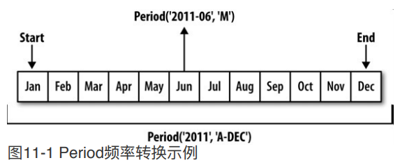
时期(period)表示的是时间区间 ,⽐如数日、数⽉、数季、数年等。(例如:p=pd.Period(2007,freq='A-DEC'),p对象表示的从2007年1⽉1⽇到2007年12⽉31⽇之间的整段时间。)
因为是时间区间,所以可以传入freq频率参数
period_range函数可⽤于创建规则的时期范围,返回的是PeriodIndex对象
既然有PeriodIndex对象,自然可以用来做Index
就像DateTimeIndex一样,DateTimeIndex索引不一定传入要DateTimeIndex对象,传入字符串组成的列表也可以
1 2 3 4 5 6 7 8 9 10 11 12 13 14 15 16 17 18 19 20 21 22 23 24 25 26 27 28 29 30 31 32 33 34 35 36 37 38 39 40 import numpy as npimport pandas as pdp = pd.Period(2007 , freq='A-DEC' ) print (p)print (p + 5 )print (p - 2 )print (pd.Period('2014' , freq='A-DEC' ) - p)rng = pd.period_range('2000-01-01' , '2000-03-30' , freq='M' ) print (rng)np.random.seed(888 ) print (pd.Series(np.random.randn(3 ), index=rng))values = ['2001Q3' , '2002Q2' , '2003Q1' ] index = pd.PeriodIndex(values, freq='Q-DEC' ) print (index)
时期的频率转换
Period和PeriodIndex对象都可以通过其asfreq⽅法被转换成别的频率。
1 2 3 4 5 6 7 8 9 10 11 12 13 14 15 import numpy as npimport pandas as pdp = pd.Period('2007' , freq='A-DEC' ) print (p)print (p.asfreq('M' , how='start' ))print (p.asfreq('M' , how='end' ))
以将Period('2007','A-DEC')看做⼀个被划分为多个⽉度时期的时间段中的游标
在A-JUN频率中:一年的范围是从7月到下一年的6月
1 2 3 4 5 6 7 8 9 10 11 12 13 14 15 import numpy as npimport pandas as pdp = pd.Period('2007' , freq='A-JUN' ) print (p)print (p.asfreq('M' , 'start' ))print (p.asfreq('M' , 'end' ))
高频率转换为低频率时,父时期(superperiod)是由子时期(subperiod)所属的位置决定的。
1 2 3 4 5 6 7 8 9 10 11 12 13 import numpy as npimport pandas as pdp = pd.Period('Aug-2007' , 'M' ) print (p)print (p.asfreq('A-JUN' ))print (p.freq)
1 2 3 4 5 6 7 8 9 10 11 12 13 14 15 16 17 18 19 20 21 22 23 24 25 26 27 28 29 30 31 32 33 34 35 36 import numpy as npimport pandas as pdnp.random.seed(888 ) rng = pd.period_range('2006' , '2009' , freq='A-DEC' ) ts = pd.Series(np.random.randn(len (rng)), index=rng) print (ts)print (ts.asfreq('M' , how='start' ))print (ts.asfreq('B' , how='end' ))print (ts.asfreq('B' , how='start' ))
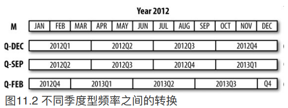
按季度计算的时期频率
pandas⽀持12种季度型频率,即QJAN到Q-DEC:
1 2 3 4 5 6 7 8 9 10 11 12 13 14 15 16 17 18 19 20 21 22 23 24 25 26 import numpy as npimport pandas as pdp = pd.Period('2012Q4' , freq='Q-JAN' ) print (p)print (p.asfreq('D' , 'start' ))print (p.asfreq('D' , 'end' ))p = pd.Period('2012Q4' , freq='Q-JAN' ) p4pm = (p.asfreq('B' , 'e' ) - 1 ).asfreq('T' , 's' ) + 16 * 60 print (p4pm)print (p4pm.to_timestamp())
period_range传入像Q-JAN一样的freq可以生成季度型范围
1 2 3 4 5 6 7 8 9 10 11 12 13 14 15 16 17 18 19 20 21 22 23 24 25 26 27 28 import numpy as npimport pandas as pdrng = pd.period_range('2011Q3' , '2012Q4' , freq='Q-JAN' ) ts = pd.Series(np.arange(len (rng)), index=rng) print (ts)new_rng = (rng.asfreq('B' , 'e' ) - 1 ).asfreq('T' , 's' ) + 16 * 60 ts.index = new_rng.to_timestamp() print (ts)
将Timestamp转换为Period(及其反向过程)
to_period()方法:时间戳索引 转换为时期索引 to_timestamp方法:
1 2 3 4 5 6 7 8 9 10 11 12 13 14 15 16 17 18 19 20 21 22 23 24 25 26 27 28 29 30 31 32 33 34 35 36 37 38 39 40 41 42 43 44 45 46 47 48 49 50 51 52 53 54 55 56 57 58 import numpy as npimport pandas as pdnp.random.seed(888 ) rng = pd.date_range('2000-01-01' , periods=3 , freq='M' ) ts = pd.Series(np.random.randn(3 ), index=rng) print (ts)print (type (ts.index))pts = ts.to_period() print (pts)print (type (pts.index))rng = pd.date_range('1/29/2000' , periods=6 , freq='D' ) ts2 = pd.Series(np.random.randn(6 ), index=rng) print (ts2)print (type (ts2.index))print (ts2.to_period('M' ))print (ts2.to_period('M' ).index)
1 2 3 4 5 6 7 8 9 10 11 12 13 14 15 16 17 18 19 20 21 22 23 24 25 26 27 28 29 30 31 32 33 import numpy as npimport pandas as pdnp.random.seed(888 ) rng = pd.date_range('1/29/2000' , periods=6 , freq='D' ) ts2 = pd.Series(np.random.randn(6 ), index=rng) print (ts2)print (type (ts2.index))ts3 = ts2.to_period('M' ) print (ts3)print (type (ts3.index))
通过数组创建PeriodIndex
有可能年度(year)和季度(quarter)不再同一列,这时就可以使用PeriodIndex的year参数和quarter参数将二者合起来,创建一个新的PeriodIndex
1 2 3 4 5 6 7 8 9 10 11 12 13 14 15 16 17 18 19 20 21 22 23 24 25 26 27 28 29 30 31 32 33 34 35 36 37 38 39 40 41 42 43 44 45 46 47 48 49 50 51 52 53 54 55 import numpy as npimport pandas as pddata = pd.read_csv('examples/macrodata.csv' ) print (data.head(3 ))print (data.year)print (data.quarter)index = pd.PeriodIndex(year=data.year, quarter=data.quarter, freq='Q-DEC' ) print (index)data.index = index print (data.infl)
11.6 重采样及频率转换 重采样(resampling)指的是将时间序列从⼀个频率转换到另⼀个频率 的处理过程。
将高频率数据聚合到低频率 称为降采样(downsampling)。
将低频率数据转换到高频率 称为升采样(upsampling)。
并不是所有的重采样都能被划分到这两个⼤类中。
升采样与降采样:
各种频率转换⼯作:resample⽅法
==resample有类似于groupby的API==,调⽤resample可以分组数据,然后会调⽤⼀个聚合函数:
1 2 3 4 5 6 7 8 9 10 11 12 13 14 15 16 17 18 19 20 21 22 23 24 25 26 27 28 29 import numpy as npimport pandas as pdrng = pd.date_range('2000-01-01' , periods=100 , freq='D' ) ts = pd.Series(np.arange(len (rng)), index=rng) print (ts)print (ts.resample('M' ).mean())print (ts.resample('M' , kind='period' ).mean())
resample⽅法的参数
降采样
使用降采样必须保证所有时间段的并集必须能组成整个时间帧 。
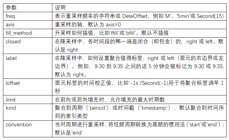
使用resample对数据进⾏降采样时,需要考虑两样东⻄:
各区间哪边是闭合的。
如何标记各个聚合⾯元,用区间的开头还是末尾。
1 2 3 4 5 6 7 8 9 10 11 12 13 14 15 16 17 18 19 20 21 22 23 24 25 26 27 28 29 30 31 32 33 34 35 36 37 38 39 40 41 42 43 44 45 46 47 48 49 50 51 52 53 54 55 56 import numpy as npimport pandas as pdrng = pd.date_range('2000-01-01' , periods=12 , freq='T' ) ts = pd.Series(np.arange(12 ), index=rng) print (ts)print (ts.resample('5min' , closed='right' ).count())print (ts.resample('5min' , closed='right' , label='right' ).count())print (ts.resample('5min' , closed='left' ).count())print (ts.resample('5min' , closed='right' ,label='right' , loffset='-1s' ).count())
closed参数说明:
label参数说明:
label参数决定索引的值
label为left的时候,就以区间左边的那个日期作为索引;label为right的时候,就以区间的右边那个日期作为索引。
loffset参数:行索引 做位移
升采样
就像前面说的,升采样时间粒度变小。例如,原来是按周统计的数据,现在变成按天统计。升采样会涉及到数据的填充
四种填充方法(实际是三种):
asfreq:ffill/pad:bfill:
1 2 3 4 5 6 7 8 9 10 11 12 13 14 15 16 17 18 19 20 21 22 23 24 25 26 27 28 29 30 31 32 33 34 35 36 37 38 39 40 41 42 43 44 45 46 47 import numpy as npimport pandas as pdrng = pd.date_range('20180101' , periods=2 ) ts = pd.Series(np.arange(2 ), index=rng) print (ts)ts_6h_asfreq = ts.resample('6H' ).asfreq() print (ts_6h_asfreq)ts_6h_pad = ts.resample('6H' ).pad() print (ts_6h_pad)ts_6h_ffill = ts.resample('6H' ).ffill() print (ts_6h_ffill)ts_6h_bfill = ts.resample('6H' ).bfill() print (ts_6h_bfill)
OHLC重采样
OHLC重采样:
使用how参数
1 2 3 4 5 6 7 8 9 10 11 12 13 14 15 16 17 18 19 20 21 22 23 24 25 26 27 28 import numpy as npimport pandas as pdrng = pd.date_range('2000-01-01' , periods=12 , freq='T' ) ts = pd.Series(np.arange(12 ), index=rng) print (ts)print (ts.resample('5min' ).ohlc())
升采样和插值
1 2 3 4 5 6 7 8 9 10 11 12 13 14 15 16 17 18 19 20 21 22 23 24 25 26 27 28 29 30 31 32 33 34 35 36 37 38 39 40 41 42 43 44 45 46 47 48 49 50 51 52 53 54 55 56 57 58 import numpy as npimport pandas as pdframe = pd.DataFrame(np.arange(10000 ,10008 ).reshape(2 ,4 ), index=pd.date_range('1/1/2000' , periods=2 ,freq='W-WED' ), columns=['Colorado' , 'Texas' , 'New York' , 'Ohio' ]) print (frame)df_daily = frame.resample('D' ).asfreq() print (df_daily)print (frame.resample('D' ).ffill())print (frame.resample('D' ).ffill(limit=2 ))print (frame.resample('W-THU' ).ffill())
通过时期进行重采样
对那些使⽤时期索引的数据进行重采样与时间戳很像:
1 2 3 4 5 6 7 8 9 10 11 12 13 14 15 16 17 18 19 20 21 22 23 24 25 26 27 28 29 30 31 32 33 34 35 36 37 38 39 40 41 42 43 44 45 import numpy as npimport pandas as pdframe = pd.DataFrame(np.arange(10000 ,10096 ).reshape(24 ,4 ), index=pd.period_range('1-2000' , '12-2001' ,freq='M' ), columns=['Colorado' , 'Texas' , 'New York' , 'Ohio' ]) print (frame[:5 ])annual_frame = frame.resample('A-DEC' ).mean() print (annual_frame)print (annual_frame.resample('Q-DEC' ).ffill())print (annual_frame.resample('Q-DEC' , convention='end' ).ffill())
由于时期指的是时间区间,所以升采样和降采样的规则就⽐较严格:
在降采样中,⽬标频率必须是源频率的子时期(subperiod)。
在升采样中,⽬标频率必须是源频率的超时期(superperiod)。
11.7 移动窗⼝函数 什么是滑动(移动)窗口?
为了提升数据的准确性,将某个点的取值扩大到包含这个点的一段区间,用区间来进行判断,这个区间就是窗口。
例如想使用2011年1月1日的一个数据,单取这个时间点的数据当然是可行的,但是太过绝对,有没有更好的办法呢?可以选取2010年12月16日到2011年1月15日,通过求均值来评估1月1日这个点的值,2010-12-16到2011-1-15就是一个窗口,窗口的长度window=30.
移动窗口就是窗口向一端滑行,每次滑动(行)并不是区间整块的滑行,而是一个单位一个单位的滑行。例如窗口2010-12-16到2011-1-15,下一个窗口并不是2011-1-15到2011-2-15,而是2010-12-17到2011-1-16 (假设数据的截取是以天为单位),==整体向右移动一个单位,而不是一个窗口==。这样统计的每个值始终都是30单位的均值。 窗口中的值从覆盖整个窗口的位置开始产生,在此之前即为NaN,举例如下:窗口大小为10,前9个都不足够为一个一个窗口的长度,因此都无法取值。
rolling函数返回的是window对象或rolling子类,可以通过调用该对象的mean(),sum(),std(),count()等函数计算返回窗口的值 ,还可以通过该对象的apply(func)函数,通过自定义函数计算窗口的特定的值
1 2 3 4 5 6 7 8 9 10 11 12 13 14 15 16 17 18 19 20 21 22 23 24 25 26 27 28 29 30 31 32 33 34 35 36 37 38 39 40 41 42 43 44 45 46 import numpy as npimport pandas as pddf = pd.DataFrame({'B' : [0 , 1 , 2 , np.nan, 4 ]}) print (df.rolling(2 ).sum ())s = [1 ,2 ,3 ,5 ,6 ,10 ,12 ,14 ,12 ,30 ] print (pd.Series(s))print (pd.Series(s).rolling(window=3 ).mean())
在移动窗口上计算的各种统计函数也是⼀类常⻅于时间序列的数组变换。这样可以圆滑噪⾳数据或断裂数据。这种函数称为移动窗口函数(moving windowfunction),其中还包括那些窗⼝不定⻓的函数(如指数加权移动平均)。跟其他统计函数⼀样,移动窗口函数也会自动排除缺失值 。
rolling运算符,它与resample和groupby很像。可以在TimeSeries或DataFrame以及⼀个window上调⽤它:
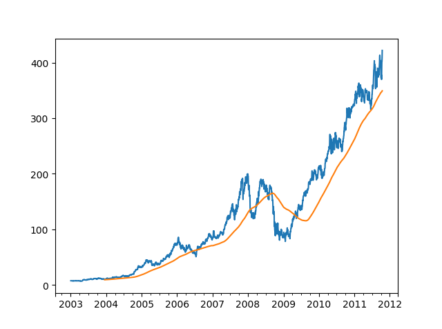
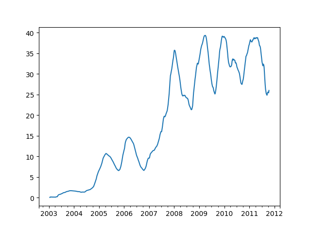
1 2 3 4 5 6 7 8 9 10 11 12 13 14 15 16 17 18 19 20 21 22 23 24 25 26 27 import numpy as npimport pandas as pdimport matplotlib.pyplot as plt close_px_all = pd.read_csv('examples/stock_px_2.csv' ,parse_dates=True , index_col=0 ) print (close_px_all.head())close_px = close_px_all[['AAPL' , 'MSFT' , 'XOM' ]] close_px = close_px.resample('B' ).ffill() print (close_px.AAPL.plot())print (close_px.AAPL.rolling(250 ).mean().plot())plt.show()
表达式rolling(250)与groupby很像,但不是对其进⾏分组、创建⼀个按照250天分组的滑动窗⼝对象 。然后,我们就得到了苹果公司股价的250天的移动窗⼝。
DataFrame.rolling(window, min_periods=None, center=False, win_type=None, on=None, axis=0, closed=None)
min_periods参数:
center参数:
win_type参数:
1 2 3 4 5 6 7 8 9 10 11 12 13 14 15 16 17 18 19 20 21 22 23 24 25 26 27 28 29 30 31 32 33 import numpy as npimport pandas as pdimport matplotlib.pyplot as plt close_px_all = pd.read_csv('examples/stock_px_2.csv' ,parse_dates=True , index_col=0 ) print (close_px_all.head())close_px = close_px_all[['AAPL' , 'MSFT' , 'XOM' ]] close_px = close_px.resample('B' ).ffill() appl_std250 = close_px.AAPL.rolling(250 , min_periods=10 ).std() print (appl_std250[5 :12 ])appl_std250.plot() plt.show()
rolling还可以接受一个指定固定⼤⼩时间补偿字符串作为一个窗口
1 2 3 4 5 6 7 8 9 10 11 12 13 14 15 16 17 18 19 20 21 22 23 24 25 26 27 28 import numpy as npimport pandas as pdimport matplotlib.pyplot as plt close_px_all = pd.read_csv('examples/stock_px_2.csv' ,parse_dates=True , index_col=0 ) print (close_px_all.head())close_px = close_px_all[['AAPL' , 'MSFT' , 'XOM' ]] close_px = close_px.resample('B' ).ffill() print (close_px.rolling('20D' ).mean())
扩展窗口:
“扩展”意味着,从时间序列的起始处开始窗口,增加窗口直到它超过所有的序列 。
DataFrame.expanding(min_periods=1, center=False, axis=0)不是固定窗口长度,其长度是不断的扩大的 。
rolling和expanding都是类似的,假设目的是查看股票市场价格随着时间的变化,不同的是rolling average算的是最近一个窗口期(比如说20天)的一个平均值,过了一天这个窗口又会向下滑动一天算20天的平均值;expanding的话,是从第一个值就开始累加地计算平均值 。
1 2 3 4 5 6 7 8 9 10 11 12 13 14 15 16 17 18 19 20 21 22 23 24 25 26 27 28 29 30 31 32 33 34 35 36 37 import numpy as npimport pandas as pddf = pd.DataFrame({'B' : [1 ,1 ,1 ,1 ,1 ,1 ,1 ,1 ]}) print (df.rolling(2 ).sum ())print (df.expanding().sum ())print (df.expanding(3 ).sum ())
指数加权函数
指数加权函数会赋予近期的观测值更大的权数 ,因此,它能适应更快的变化
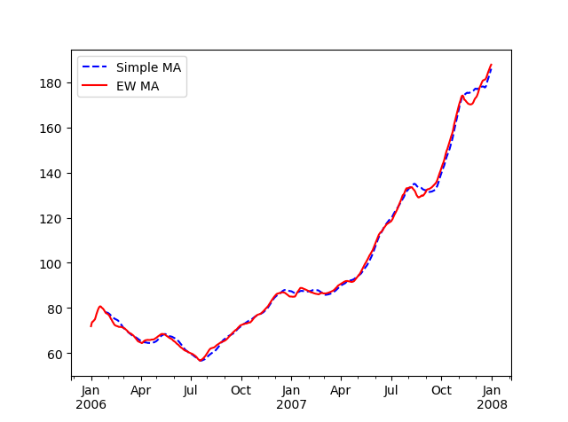
1 2 3 4 5 6 7 8 9 10 11 12 13 14 15 16 17 18 19 20 21 22 23 24 25 26 27 28 29 30 31 32 33 import numpy as npimport pandas as pdimport matplotlib.pyplot as plt close_px_all = pd.read_csv('examples/stock_px_2.csv' ,parse_dates=True , index_col=0 ) print (close_px_all.head())close_px = close_px_all[['AAPL' , 'MSFT' , 'XOM' ]] close_px = close_px.resample('B' ).ffill() aapl_px = close_px.AAPL['2006' :'2007' ] ma60 = aapl_px.rolling(30 , min_periods=20 ).mean() ewma60 = aapl_px.ewm(span=30 ).mean() ma60.plot(style='b--' , label='Simple MA' ) ewma60.plot(style='r-' , label='EW MA' ) plt.legend() plt.show()
⼆元移动窗口函数
一些统计计算符,比如相关性和协方差,需要在两个时间序列上进行计算。
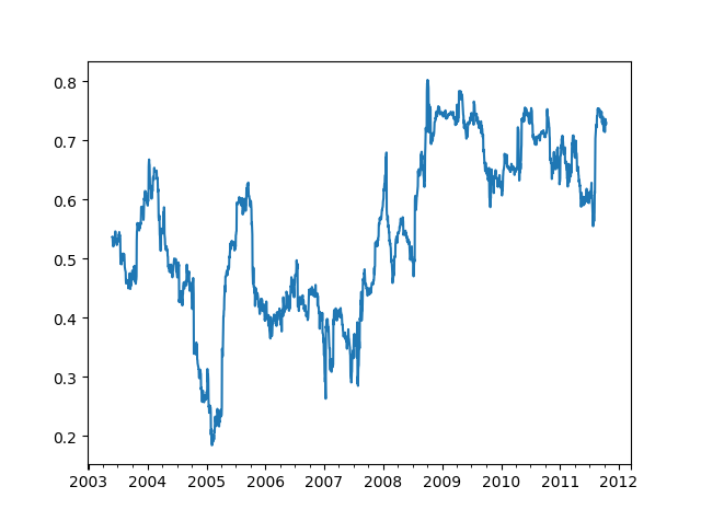
1 2 3 4 5 6 7 8 9 10 11 12 13 14 15 16 17 18 19 20 21 22 23 24 25 26 27 28 29 30 31 32 33 34 35 36 37 38 39 40 41 42 43 44 45 46 47 48 49 50 51 52 53 54 55 56 57 58 59 60 61 62 63 64 65 import numpy as npimport pandas as pdimport matplotlib.pyplot as plt close_px_all = pd.read_csv('examples/stock_px_2.csv' ,parse_dates=True , index_col=0 ) print (close_px_all.head())close_px = close_px_all[['AAPL' , 'MSFT' , 'XOM' ]] close_px = close_px.resample('B' ).ffill() spx_px = close_px_all['SPX' ] print (spx_px.head())print (close_px.head())spx_rets = spx_px.pct_change() returns = close_px.pct_change() print (spx_rets.head())print (returns.head())corr = returns.AAPL.rolling(125 , min_periods=100 ).corr(spx_rets) corr.plot() plt.show()
⽤户定义的移动窗口函数
通过rolling().apply()方法,可以在移动窗口上使用自己定义的函数。唯一需要满足的是,在数组的每一个片段上,函数必须产生单个值 。
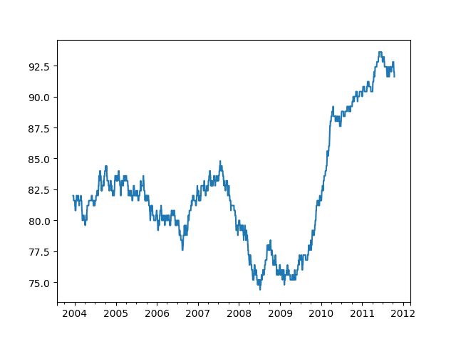
1 2 3 4 5 6 7 8 9 10 11 12 13 14 15 16 17 18 19 20 21 22 23 24 25 26 27 28 29 30 31 32 33 34 35 36 37 38 39 import numpy as npimport pandas as pdimport matplotlib.pyplot as plt from scipy.stats import percentileofscoreclose_px_all = pd.read_csv('examples/stock_px_2.csv' ,parse_dates=True , index_col=0 ) close_px = close_px_all[['AAPL' , 'MSFT' , 'XOM' ]].resample('B' ).ffill() print (close_px.head())returns = close_px.pct_change() print (returns.head())score_at_2percent = lambda x: percentileofscore(x, 0.02 ) result = returns.AAPL.rolling(250 ).apply(score_at_2percent) result.plot() plt.show()