# 不能通过传入字典的方式作为index来创建多层索引 data = pd.Series(np.random.randn(9), index={'a':[1,2,3],'b':[1,3],'c':[1,2],'d':[2,3]}) # ValueError: Length of passed values is 9, index implies 4
print(df) # state Ohio Colorado # color Green Red Green # floor1 floor2 # a 1 10000 10001 10002 # 2 10003 10004 10005 # b 1 10006 10007 10008 # 2 10009 10010 10011
print(df['Ohio']) # color Green Red # floor1 floor2 # a 1 10000 10001 # 2 10003 10004 # b 1 10006 10007 # 2 10009 10010
print(df) # state Ohio Colorado # color Green Red Green # floor1 floor2 # a 1 10000 10001 10002 # 2 10003 10004 10005 # b 1 10006 10007 10008 # 2 10009 10010 10011
print(df2) # state Ohio Colorado # color Green Red Green # floor2 floor1 # 1 a 10000 10001 10002 # 2 a 10003 10004 10005 # 1 b 10006 10007 10008 # 2 b 10009 10010 10011
# 根据单个级别中的值对数据进⾏排序 print(df.sort_index(level=1)) # state Ohio Colorado # color Green Red Green # floor1 floor2 # a 1 10000 10001 10002 # b 1 10006 10007 10008 # a 2 10003 10004 10005 # b 2 10009 10010 10011
# 交换floor2和floor1位置后,再根据值来排序 print(df.swaplevel(0, 1).sort_index(level=0)) # state Ohio Colorado # color Green Red Green # floor2 floor1 # 1 a 10000 10001 10002 # b 10006 10007 10008 # 2 a 10003 10004 10005 # b 10009 10010 10011
print(df) # state Ohio Colorado # color Green Red Green # floor1 floor2 # a 1 10000 10001 10002 # 2 10003 10004 10005 # b 1 10006 10007 10008 # 2 10009 10010 10011
# 当是多重索引的时候,可以使用level来合并数据 print(df.sum(level='floor1')) # state Ohio Colorado # color Green Red Green # floor1 # a 20003 20005 20007 # b 20015 20017 20019
print(df.sum(level='floor2')) # state Ohio Colorado # color Green Red Green # floor2 # 1 20006 20008 20010 # 2 20012 20014 20016
print(df.sum(level='color', axis=1)) # color Green Red # floor1 floor2 # a 1 20002 10001 # 2 20008 10004 # b 1 20014 10007 # 2 20020 10010
print(frame) # a b c d # 0 0 7 one 0 # 1 1 6 one 1 # 2 2 5 one 2 # 3 3 4 two 0 # 4 4 3 two 1 # 5 5 2 two 2 # 6 6 1 two 3
frame2 = frame.set_index(['c', 'd']) print(frame2) # a b # c d # one 0 0 7 # 1 1 6 # 2 2 5 # two 0 3 4 # 1 4 3 # 2 5 2 # 3 6 1
frame3 = frame.set_index(['c', 'd'],drop=False) print(frame3) # a b c d # c d # one 0 0 7 one 0 # 1 1 6 one 1 # 2 2 5 one 2 # two 0 3 4 two 0 # 1 4 3 two 1 # 2 5 2 two 2 # 3 6 1 two 3
# 不管原来的Index是什么,全部都会变成RangeIndex print(frame2.reset_index()) # c d a b # 0 one 0 0 7 # 1 one 1 1 6 # 2 one 2 2 5 # 3 two 0 3 4 # 4 two 1 4 3 # 5 two 2 5 2 # 6 two 3 6 1
print(df1) # key data1 # 0 b 0 # 1 b 1 # 2 a 2 # 3 c 3 # 4 a 4 # 5 a 5 # 6 b 6
print(df2) # key data2 # 0 a 0 # 1 b 1 # 2 d 2
# 就是数据库中的一对多的join链接 # df2为一,df1为多,默认inner join on # 如果不指定on参数,就会将重叠列的列名作为键 print(pd.merge(df1, df2)) # key data1 data2 # 0 b 0 1 # 1 b 1 1 # 2 b 6 1 # 3 a 2 0 # 4 a 4 0 # 5 a 5 0
# 明确指定join on的列 print(pd.merge(df1, df2,on='key')) # key data1 data2 # 0 b 0 1 # 1 b 1 1 # 2 b 6 1 # 3 a 2 0 # 4 a 4 0 # 5 a 5 0
# 全外连接 print(pd.merge(df1, df2,on='key',how='outer')) # key data1 data2 # 0 b 0.0 1.0 # 1 b 1.0 1.0 # 2 b 6.0 1.0 # 3 a 2.0 0.0 # 4 a 4.0 0.0 # 5 a 5.0 0.0 # 6 c 3.0 NaN # 7 d NaN 2.0
print(df3) # lkey data1 # 0 b 0 # 1 b 1 # 2 a 2 # 3 c 3 # 4 a 4 # 5 a 5 # 6 b 6
print(df4) # rkey data2 # 0 a 0 # 1 b 1 # 2 d 2
# 两个列的列名不同,使用left_on和right_on指定 # 下面代码用SQL解释为: # df3 inner join df4 on df3.lkey = df4.rkey df = pd.merge(df3, df4, left_on='lkey', right_on='rkey') print(df) # lkey data1 rkey data2 # 0 b 0 b 1 # 1 b 1 b 1 # 2 b 6 b 1 # 3 a 2 a 0 # 4 a 4 a 0 # 5 a 5 a 0
left = pd.DataFrame({'key1': ['foo', 'foo', 'bar'], 'key2': ['one', 'two', 'one'], 'lval': [1, 2, 3]}) right = pd.DataFrame({'key1': ['foo', 'foo', 'bar', 'bar'], 'key2': ['one', 'one', 'one', 'two'], 'rval': [4, 5, 6, 7]}) print(left) # key1 key2 lval # 0 foo one 1 # 1 foo two 2 # 2 bar one 3
print(right) # key1 key2 rval # 0 foo one 4 # 1 foo one 5 # 2 bar one 6 # 3 bar two 7
print(pd.merge(left, right, on='key1')) # key1 key2_x lval key2_y rval # 0 foo one 1 one 4 # 1 foo one 1 one 5 # 2 foo two 2 one 4 # 3 foo two 2 one 5 # 4 bar one 3 one 6 # 5 bar one 3 two 7
print(pd.merge(left, right, on='key1', suffixes=('_left', '_right'))) # key1 key2_left lval key2_right rval # 0 foo one 1 one 4 # 1 foo one 1 one 5 # 2 foo two 2 one 4 # 3 foo two 2 one 5 # 4 bar one 3 one 6 # 5 bar one 3 two 7
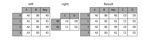
print(left2) # Ohio Nevada # a 1.0 2.0 # c 3.0 4.0 # e 5.0 6.0
print(right2) # Missouri Alabama # b 7.0 8.0 # c 9.0 10.0 # d 11.0 12.0 # e 13.0 14.0
# 双方都使用index作为连接键 print(pd.merge(left2, right2, how='outer', left_index=True, right_index=True)) # Ohio Nevada Missouri Alabama # a 1.0 2.0 NaN NaN # b NaN NaN 7.0 8.0 # c 3.0 4.0 9.0 10.0 # d NaN NaN 11.0 12.0 # e 5.0 6.0 13.0 14.0
print(left2) # Ohio Nevada # a 1.0 2.0 # c 3.0 4.0 # e 5.0 6.0
print(right2) # Missouri Alabama # b 7.0 8.0 # c 9.0 10.0 # d 11.0 12.0 # e 13.0 14.0
print(another) # New York Oregon # a 7.0 8.0 # c 9.0 10.0 # e 11.0 12.0 # f 16.0 17.0
print(left2.join([right2, another])) # Ohio Nevada Missouri Alabama New York Oregon # a 1.0 2.0 NaN NaN 7.0 8.0 # c 3.0 4.0 9.0 10.0 9.0 10.0 # e 5.0 6.0 13.0 14.0 11.0 12.0
print(left2.join([right2, another], how='outer')) # Ohio Nevada Missouri Alabama New York Oregon # a 1.0 2.0 NaN NaN 7.0 8.0 # b NaN NaN 7.0 8.0 NaN NaN # c 3.0 4.0 9.0 10.0 9.0 10.0 # d NaN NaN 11.0 12.0 NaN NaN # e 5.0 6.0 13.0 14.0 11.0 12.0 # f NaN NaN NaN NaN 16.0 17.0
print(left1) # key value # 0 a 0 # 1 b 1 # 2 a 2 # 3 a 3 # 4 b 4 # 5 c 5
print(right1) # group_val # a 3.5 # b 7.0
# 把右图的index和左图的key列进行连接 print(left1.join(right1, on='key')) # key value group_val # 0 a 0 3.5 # 1 b 1 7.0 # 2 a 2 3.5 # 3 a 3 3.5 # 4 b 4 7.0 # 5 c 5 NaN
# 没有on参数的情况下只会查找两个表的行索引,不管列有没有重叠 # 这里因为没有相同或相似的列,所以group_val为NaN print(left1.join(right1)) # key value group_val # 0 a 0 NaN # 1 b 1 NaN # 2 a 2 NaN # 3 a 3 NaN # 4 b 4 NaN # 5 c 5 NaN
print(left2) # Ohio Nevada # a 1.0 2.0 # c 3.0 4.0 # e 5.0 6.0
print(right2) # Missouri Alabama # b 7.0 8.0 # c 9.0 10.0 # d 11.0 12.0 # e 13.0 14.0
# 使用merge的left_index和right_index参数 print(pd.merge(left2, right2, how='outer', left_index=True, right_index=True)) # Ohio Nevada Missouri Alabama # a 1.0 2.0 NaN NaN # b NaN NaN 7.0 8.0 # c 3.0 4.0 9.0 10.0 # d NaN NaN 11.0 12.0 # e 5.0 6.0 13.0 14.0
# 使用DataFrame(left2)的实例方法join # 因为没有on参数,会比较两个表的行索引值来进行join print(left2.join(right2, how='outer')) # Ohio Nevada Missouri Alabama # a 1.0 2.0 NaN NaN # b NaN NaN 7.0 8.0 # c 3.0 4.0 9.0 10.0 # d NaN NaN 11.0 12.0 # e 5.0 6.0 13.0 14.0
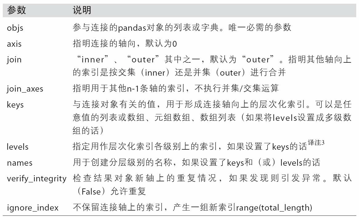
print(pd.concat([s1, s4], axis=1)) # 0 1 # a 0.0 0 # b 1.0 1 # f NaN 5 # g NaN 6
print(pd.concat([s1, s4], axis=1, join='inner')) # 0 1 # a 0 0 # b 1 1
# 指定索引名称:join_axes(指定要在其它轴上使⽤的索引) print(pd.concat([s1, s4], axis=1, join_axes=[['a', 'c', 'b', 'e']])) # 0 1 # a 0.0 0.0 # c NaN NaN # b 1.0 1.0 # e NaN NaN
print(pd.concat([s1, s1, s3])) # a 0 # b 1 # a 0 # b 1 # f 5 # g 6 # dtype: int64
# key:创建多级索引.会将每个表制作成一个外层 result = pd.concat([s1, s1, s3], keys=['one', 'two', 'three']) print(result) # one a 0 # b 1 # two a 0 # b 1 # three f 5 # g 6 # dtype: int64
print(result.unstack()) # a b f g # one 0.0 1.0 NaN NaN # two 0.0 1.0 NaN NaN # three NaN NaN 5.0 6.0
df1 = pd.DataFrame(np.arange(6).reshape(3, 2), index=['a', 'b', 'c'], columns=['one', 'two']) df2 = pd.DataFrame(5 + np.arange(4).reshape(2, 2), index=['a', 'c'], columns=['three', 'four']) print(df1) # one two # a 0 1 # b 2 3 # c 4 5
print(df2) # three four # a 5 6 # c 7 8
# 使用key参数创建多级索引 print(pd.concat([df1, df2], axis=1, keys=['level1', 'level2'])) # level1 level2 # one two three four # a 0 1 5.0 6.0 # b 2 3 NaN NaN # c 4 5 7.0 8.0
# 传入的两个表是dict形式的话,也会创建多级列表 print(pd.concat({'level1': df1, 'level2': df2}, axis=1)) # level1 level2 # one two three four # a 0 1 5.0 6.0 # b 2 3 NaN NaN # c 4 5 7.0 8.0
data = pd.DataFrame(np.arange(6).reshape((2, 3)), index=pd.Index(['Ohio', 'Colorado'], name='state'), columns=pd.Index(['one', 'two', 'three'],name='number'))
print(data) # number one two three # state # Ohio 0 1 2 # Colorado 3 4 5
# 一维表转为二维表 # 默认情况下,stack操作的是最内层. result = data.stack() print(result) # state number # Ohio one 0 # two 1 # three 2 # Colorado one 3 # two 4 # three 5 # dtype: int32
# 二维表转为一维表 # # 默认情况下,unstack操作的是最内层. print(result.unstack()) # number one two three # state # Ohio 0 1 2 # Colorado 3 4 5
print(result.unstack(level=0)) # state Ohio Colorado # number # one 0 3 # two 1 4 # three 2 5
print(result.unstack(level=1)) # number one two three # state # Ohio 0 1 2 # Colorado 3 4 5 # state Ohio Colorado
print(result.unstack(level='state')) # state Ohio Colorado # number # one 0 3 # two 1 4 # three 2 5
data = pd.DataFrame(np.arange(6).reshape((2, 3)), index=pd.Index(['Ohio', 'Colorado'], name='state'), columns=pd.Index(['one', 'two', 'three'],name='number'))
print(data) # number one two three # state # Ohio 0 1 2 # Colorado 3 4 5
# 一维表转为二维表 # 默认情况下,stack操作的是最内层. result = data.stack() print(result) # state number # Ohio one 0 # two 1 # three 2 # Colorado one 3 # two 4 # three 5 # dtype: int32
df = pd.DataFrame({'left': result, 'right': result + 5}, columns=pd.Index(['left', 'right'], name='side')) print(df) # side left right # state number # Ohio one 0 5 # two 1 6 # three 2 7 # Colorado one 3 8 # two 4 9 # three 5 10
# 在对DataFrame进⾏unstack操作时,作为旋转轴的级别将会成为结果中的最低级别 print(df.unstack('state')) # side left right # state Ohio Colorado Ohio Colorado # number # one 0 3 5 8 # two 1 4 6 9 # three 2 5 7 10
print(df.unstack('state').stack('side')) # state Colorado Ohio # number side # one left 3 0 # right 8 5 # two left 4 1 # right 9 6 # three left 5 2 # right 10 7
import numpy as np import pandas as pd from pandas import Series, DataFrame
np.random.seed(666)
# series reindex s1 = Series([1, 2, 3, 4], index=['A', 'B', 'C', 'D']) print(s1) ''' A 1 B 2 C 3 D 4 dtype: int64 '''
# 重新指定 index, 多出来的index,可以使用fill_value 填充 print(s1.reindex(index=['A', 'B', 'C', 'D', 'E'], fill_value = 10)) ''' A 1 B 2 C 3 D 4 E 10 dtype: int64 '''
s2 = Series(['A', 'B', 'C'], index = [1, 5, 10]) print(s2) ''' 1 A 5 B 10 C dtype: object '''
# 修改索引, # 将s2的索引增加到15个 # 如果新增加的索引值不存在,默认为 Nan print(s2.reindex(index=range(15))) ''' 0 NaN 1 A 2 NaN 3 NaN 4 NaN 5 B 6 NaN 7 NaN 8 NaN 9 NaN 10 C 11 NaN 12 NaN 13 NaN 14 NaN dtype: object '''
# ffill : foreaward fill 向前填充, # 如果新增加索引的值不存在,那么按照前一个非nan的值填充进去 print(s2.reindex(index=range(15), method='ffill')) ''' 0 NaN 1 A 2 A 3 A 4 A 5 B 6 B 7 B 8 B 9 B 10 C 11 C 12 C 13 C 14 C dtype: object '''
# 为 dataframe 添加一个新的索引 # 可以看到 自动 扩充为 nan print(df1.reindex(index=['A', 'B', 'C', 'D', 'E', 'F'])) ''' 自动填充为 nan c1 c2 c3 c4 c5 A 0.700437 0.844187 0.676514 0.727858 0.951458 B 0.012703 0.413588 0.048813 0.099929 0.508066 C NaN NaN NaN NaN NaN D 0.200248 0.744154 0.192892 0.700845 0.293228 E 0.774479 0.005109 0.112858 0.110954 0.247668 F 0.023236 0.727321 0.340035 0.197503 0.909180 '''
# 扩充列, 也是一样的 print(df1.reindex(columns=['c1', 'c2', 'c3', 'c4', 'c5', 'c6'])) ''' c1 c2 c3 c4 c5 c6 A 0.700437 0.844187 0.676514 0.727858 0.951458 NaN B 0.012703 0.413588 0.048813 0.099929 0.508066 NaN D 0.200248 0.744154 0.192892 0.700845 0.293228 NaN E 0.774479 0.005109 0.112858 0.110954 0.247668 NaN F 0.023236 0.727321 0.340035 0.197503 0.909180 NaN '''
# 减小 index print(s1.reindex(['A', 'B'])) ''' 相当于一个切割效果 A 1 B 2 dtype: int64 '''
# melt:逆透视 # id_vars:不需要转换的列 melted = pd.melt(df, id_vars=['key']) print(melted) # key variable value # 0 foo A 1 # 1 bar A 2 # 2 baz A 3 # 3 foo B 4 # 4 bar B 5 # 5 baz B 6 # 6 foo C 7 # 7 bar C 8 # 8 baz C 9
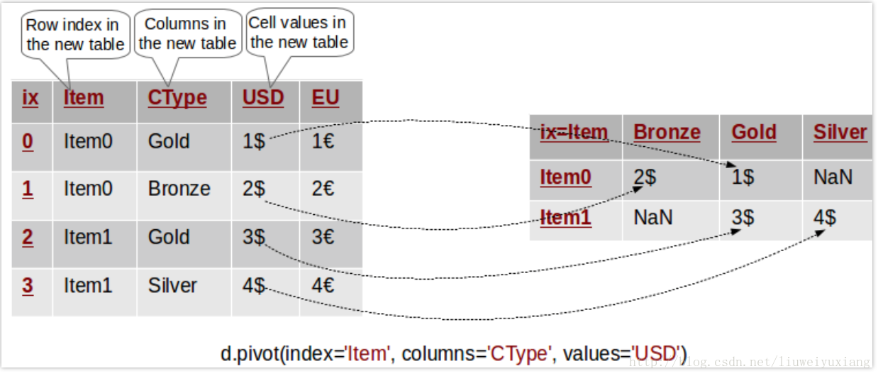
# pivot:数据透视 reshaped = melted.pivot('key', 'variable', 'value') print(reshaped) # variable A B C # key # bar 2 5 8 # baz 3 6 9 # foo 1 4 7
# pivot数据透视其实也是一种创建索引的过程 # 所以可以使用set_index复原 print(reshaped.reset_index()) # variable key A B C # 0 bar 2 5 8 # 1 baz 3 6 9 # 2 foo 1 4 7
# id_vars:不需要被转换的列名 # value_vars:需要转换的列名 print(pd.melt(df, id_vars=['key'], value_vars=['A', 'B'])) # key variable value # 0 foo A 1 # 1 bar A 2 # 2 baz A 3 # 3 foo B 4 # 4 bar B 5 # 5 baz B 6
# value_vars:需要转换的列名 print(pd.melt(df, value_vars=['A', 'B', 'C'])) # variable value # 0 A 1 # 1 A 2 # 2 A 3 # 3 B 4 # 4 B 5 # 5 B 6 # 6 C 7 # 7 C 8 # 8 C 9
# value_vars:需要转换的列名 print(pd.melt(df, value_vars=['key', 'A', 'B'])) # variable value # 0 key foo # 1 key bar # 2 key baz # 3 A 1 # 4 A 2 # 5 A 3 # 6 B 4 # 7 B 5 # 8 B 6