第14章 数据分析案例
14.1 来⾃Bitly的USA.gov数据
读取json数据:
1 | import json |
⽤纯Python代码对时区进⾏计数
1 | import json |
⽤pandas对时区进⾏计数
1 | import json |
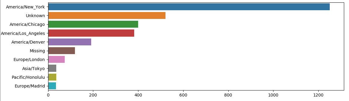
我们可以⽤matplotlib可视化这个数据
1 | import seaborn as sns |
继续做后续处理:
1 | # 将a列截短一点 |
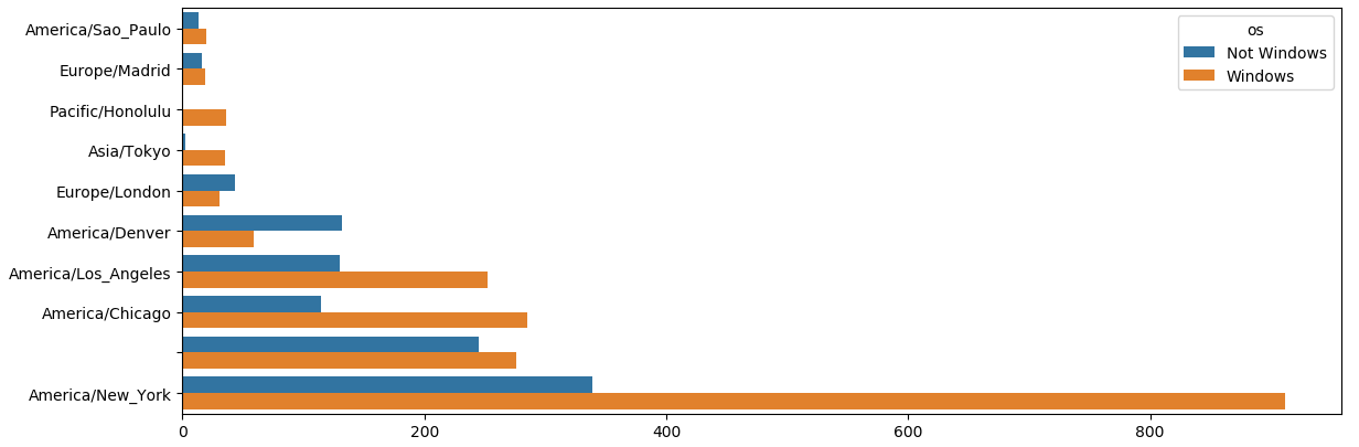
我们将数据制作成图:
1 | # 重新排列数据以便绘图 |
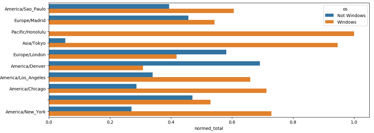
最常出现时区的Windows和⾮Windows⽤户的百分⽐
1 | def norm_total(group): |
14.2 MovieLens 1M数据集
数据准备:
1 | import pandas as pd |
女性最喜欢的电影:
1 | # merge函数将ratings跟users合并到⼀起,然后再将movies也合并进去。 |
计算评分分歧
假设我们想要找出男性和⼥性观众分歧最⼤的电影。⼀个办法是给mean_ratings加上⼀个⽤于存放平均得分之差的列,并对其进⾏排序:
1 | mean_ratings['diff'] = mean_ratings['M'] - mean_ratings['F'] |
求标准差:
1 | # 按标题分组的评级标准差 |