第12章 pandas⾼级应⽤ 前⾯的章节关注于不同类型的数据规整流程和NumPy、pandas与其它库的特点。本章就要深⼊学习pandas的⾼级功能。
12.1 分类数据 使用分类数据提⾼性能 和内存的使⽤率 。
背景和⽬的
Series和Datatime难免会拥有重复数据,MySQL是如何处理重复数据的?使用外键.将主要的参数存储为引⽤维表整数键,
⽤整数表示的⽅法称为分类或字典编码表示法
1
2
3
4
5
6
7
8
9
10
11
12
13
14
15
16
17
18
19
20
21
22
23
24
25
26
27
28
29
30
31
32
33
34
35
36
37
38
39
40
41
42
43
44
45
46
47
48
49
50
51
52
53
54
55
56
57
58
59
60
61
62
63
64
65
import numpy as npimport pandas as pdvalues = pd.Series(['apple' , 'orange' , 'apple' ,'apple' ] * 2 ) print (values)print (pd.unique(values))print (pd.value_counts(values))values = pd.Series([0 , 1 , 0 , 0 ] * 2 ) dim = pd.Series(['apple' , 'orange' ]) print (values)print (dim)print (dim.take([0 ,1 ]))print (dim.take(values))
pandas的分类类型
⽤于保存使⽤整数分类表示法的数据。
Categories对象:
构造函数pd.Categorical()
第二种构造函数pd.Categorical.from_codes():分类编码(Categories对象的codes属性)和分类数据
在创建Categories对象的时候,from_codes构造器能够使用ordered参数实现对分类的排序
对于已经存在的Categories对象,可以使用as_ordered()方法实现对分类的排序
对于Series和DataFrame对象,可以使用astype('category')将列转为Categories对象
1
2
3
4
5
6
7
8
9
10
11
12
13
14
15
16
17
18
19
20
21
22
23
24
25
26
27
28
29
30
31
32
33
34
35
36
37
38
39
40
import numpy as npimport pandas as pdmy_categories = pd.Categorical(['foo' , 'bar' , 'baz' , 'foo' , 'bar' ]) print (my_categories)print (my_categories.categories)print (my_categories.codes)categories = ['foo' , 'bar' , 'baz' ] codes = [0 , 1 , 2 , 0 , 0 , 1 ] my_cats_2 = pd.Categorical.from_codes(codes, categories) print (my_cats_2)ordered_cat = pd.Categorical.from_codes(codes, categories,ordered=True ) print (ordered_cat)print (my_cats_2.as_ordered())
1
2
3
4
5
6
7
8
9
10
11
12
13
14
15
16
17
18
19
20
21
22
23
24
25
26
27
28
29
30
31
32
33
34
35
36
37
38
39
40
41
42
43
44
45
46
47
48
49
50
51
52
53
54
55
56
57
58
59
60
61
62
63
import numpy as npimport pandas as pdnp.random.seed(888 ) fruits = ['apple' , 'orange' , 'apple' , 'apple' ] * 2 N = len (fruits) df = pd.DataFrame({'fruit' : fruits, 'basket_id' : np.arange(N), 'count' : np.random.randint(3 , 15 , size=N), 'weight' : np.random.uniform(0 , 4 , size=N)}, columns=['basket_id' , 'fruit' , 'count' , 'weight' ]) print (df)fruit_cat = df['fruit' ].astype('category' ) print (fruit_cat)print (type (fruit_cat))c = fruit_cat.values print (type (c))df['fruit' ] = df['fruit' ].astype('category' ) print (df.fruit)
⽤分类进⾏计算
使⽤pandas.qcut⾯元函数。它会返回pandas.Categorical对象
使用pandas.qcut函数的labels参数:
可以将Categorical对象制作成Series对象,然后传给DataFrame的groupby函数,实现分组聚合.
也可以直接将Categorical对象传给groupby函数,实现分组聚合.
1
2
3
4
5
6
7
8
9
10
11
12
13
14
15
16
17
18
19
20
21
22
23
24
25
26
27
28
29
30
31
32
33
34
35
36
37
38
39
40
41
42
43
44
45
46
47
48
49
50
51
52
53
54
55
import numpy as npimport pandas as pdnp.random.seed(12345 ) draws = np.random.randn(1000 ) print (draws[:5 ])bins = pd.qcut(draws, 4 ) print (bins)print (type (bins))bins = pd.qcut(draws, 4 , labels=['Q1' , 'Q2' , 'Q3' , 'Q4' ]) print (bins)print (bins.codes[:10 ])bins = pd.Series(bins, name='quartile' ) print (bins.head())results = (pd.Series(draws) .groupby(bins) .agg(['count' , 'min' , 'max' ]) .reset_index()) print (results)
直接将Categorical对象传给groupby函数,实现分组聚合:
1
2
3
4
5
6
7
8
9
10
11
12
13
14
15
16
17
18
19
20
21
22
23
24
25
26
27
28
import numpy as npimport pandas as pdnp.random.seed(12345 ) draws = np.random.randn(1000 ) bins = pd.qcut(draws, 4 ) bins = pd.qcut(draws, 4 , labels=['Q1' , 'Q2' , 'Q3' , 'Q4' ]) print (bins)results = (pd.Series(draws) .groupby(bins) .agg(['count' , 'min' , 'max' ]) .reset_index()) print (results)
⽤分类提⾼性能
如果你是在⼀个特定数据集上做⼤量分析,将其转换为分类可以极⼤地提⾼效率
分类比标签快
GroupBy操作⽐分类快
1
2
3
4
5
6
7
8
9
10
11
12
13
14
15
16
17
18
import numpy as npimport pandas as pdnp.random.seed(888 ) N = 10000000 draws = pd.Series(np.random.randn(N)) labels = pd.Series(['foo' , 'bar' , 'baz' , 'qux' ] * (N // 4 )) categories = labels.astype('category' ) print (labels.memory_usage())print (categories.memory_usage())
分类⽅法
包含分类数据的Series 有⼀些特殊的⽅法,类似于Series.str字符串⽅法。
包含分类数据的Series的cat属性提供了分类⽅法的⼊⼝
Categories()创建分类对象,Series.astype('category')将列转换为分类对象,Series.cat.set_categories在旧类别的基础上创建新类别或移除部分旧类别remove_unused_categories⽅法删除没有使用到的分类
1
2
3
4
5
6
7
8
9
10
11
12
13
14
15
16
17
18
19
20
21
22
23
24
25
26
27
28
29
30
31
32
33
34
35
36
37
38
39
40
41
42
43
44
45
46
47
48
49
50
51
52
53
54
55
56
57
58
59
60
61
62
63
64
65
66
67
68
69
70
71
72
73
74
75
76
77
78
79
80
81
82
83
84
85
86
87
88
89
90
91
92
93
94
95
96
97
98
99
100
101
import numpy as npimport pandas as pds = pd.Series(['a' , 'b' , 'c' , 'd' ] * 2 ) cat_s = s.astype('category' ) print (cat_s)print (cat_s.cat.codes)print (cat_s.cat.categories)actual_categories = ['a' , 'b' , 'c' , 'd' , 'e' ] cat_s2 = cat_s.cat.set_categories(actual_categories) print (cat_s2)print (cat_s.value_counts())print (cat_s2.value_counts())print (cat_s.isin(['a' , 'b' ]))cat_s3 = cat_s[cat_s.isin(['a' , 'b' ])] print (cat_s3)print (cat_s3.cat.remove_unused_categories())
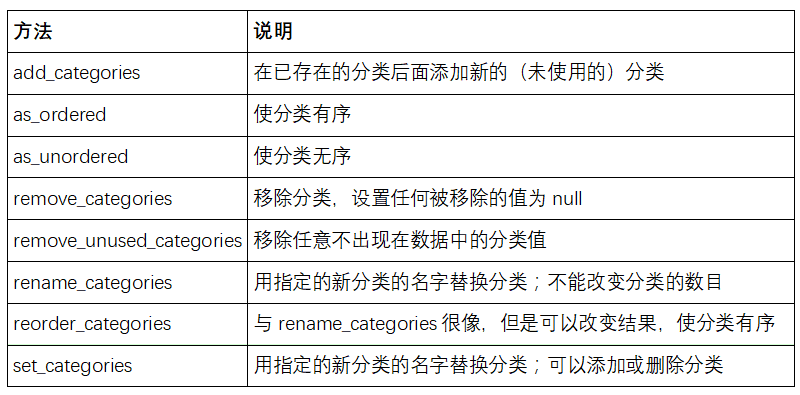
cat属性的方法
为建模创建虚拟变量
当你使⽤统计或机器学习⼯具时,通常会将分类数据转换为虚拟变量,也称为one-hot编码。这包括创建⼀个不同类别的列的DataFrame;这些列包含给定分类的1,其它为0。
pandas.get_dummies函数可以把分类数据转换为包含虚拟变量的DataFrame:
1
2
3
4
5
6
7
8
9
10
11
12
13
14
15
16
17
18
19
20
21
22
23
24
25
26
27
28
29
import numpy as npimport pandas as pdcat_s = pd.Series(['a' , 'b' , 'c' , 'd' ] * 2 , dtype='category' ) print (cat_s)print (pd.get_dummies(cat_s))
12.2 GroupBy⾼级应⽤ 分组转换和“解封”GroupBy
apply为DataFrame的轴级应用函数.
transform⽅法:
它可以产⽣向分组形状⼴播标量值
它可以产⽣⼀个和输⼊组形状相同的对象
它不能修改输⼊
简单来说transform方法和普通GroupBy方法最大的不同:
1
2
3
4
5
6
7
8
9
10
11
12
13
14
15
16
17
18
19
20
21
22
23
24
25
26
27
28
29
30
31
32
33
34
35
36
37
38
39
40
41
42
43
44
45
46
47
48
49
50
51
52
53
54
55
56
57
58
59
60
61
62
63
64
65
66
67
68
69
70
71
72
73
74
75
76
77
78
79
80
81
82
83
84
85
86
87
88
89
90
91
92
93
94
95
96
97
98
99
100
101
102
103
104
105
106
107
108
109
110
111
112
113
114
115
116
117
118
119
120
121
122
123
124
125
126
127
128
129
130
131
132
133
134
135
136
137
138
139
140
141
142
143
144
145
146
147
148
149
150
151
152
153
154
155
156
157
158
159
160
161
162
163
164
165
166
167
168
169
170
import pandas as pdimport numpy as npdf = pd.DataFrame({'key' : ['a' , 'b' , 'c' ] * 4 , 'value' : np.arange(12. )}) print (df)g = df.groupby('key' ).value print (g.mean())print (g.transform(lambda x: x.mean()))print (g.transform('mean' ))print (g.transform(lambda x: x * 2 ))print (g.transform(lambda x: x.rank(ascending=False )))def normalize (x ): return (x - x.mean()) / x.std() print (g.transform(normalize))print (g.apply(normalize))print (g.transform('mean' ))normalized = (df['value' ] - g.transform('mean' )) / g.transform('std' ) print (normalized)
分组的时间重采样
对于时间序列数据,resample⽅法从语义上是⼀个基于内在时间的分组操作。
使用pandas.TimeGrouper对象:时间必须是Series或DataFrame的索引 。
1
2
3
4
5
6
7
8
9
10
11
12
13
14
15
16
17
18
19
20
21
22
23
24
25
26
27
28
29
30
31
32
33
34
35
36
37
38
39
40
41
42
43
44
45
46
47
48
49
50
51
52
53
54
55
56
57
58
59
60
61
62
63
64
65
66
67
68
69
70
71
72
73
74
75
76
77
78
79
80
81
82
83
import pandas as pdimport numpy as npN = 15 times = pd.date_range('2017-05-20 00:00' , freq='1min' , periods=N) df = pd.DataFrame({'time' : times,'value' : np.arange(N)}) print (df)print (df.set_index('time' ).resample('5min' ).count())df2 = pd.DataFrame({'time' : times.repeat(3 ), 'key' : np.tile(['a' , 'b' , 'c' ], N), 'value' : np.arange(N * 3. )}) print (df2[:7 ])time_key = pd.TimeGrouper('5min' ) resampled = (df2.set_index('time' ) .groupby(['key' , time_key]) .sum ()) print (resampled)print (resampled.reset_index())
12.3 链式编程技术 当对数据集进⾏⼀系列变换时,可能创建的多个临时变量其实并没有在分析中⽤到。
1
2
3
4
5
6
7
8
import numpy as npimport pandas as pddf = load_data() df2 = df[df['col2' ] < 0 ] df2['col1_demeaned' ] = df2['col1' ] - df2['col1' ].mean() result = df2.groupby('key' ).col1_demeaned.std()
使用DataFrame.assign:
DataFrame.assign⽅法是⼀个df[k] = v形式的函数式的列分配⽅法。它不是就地修改对象,⽽是返回新的修改过的DataFrame
下面两个语句是等价的
1
2
3
4
5
6
7
8
9
10
11
import numpy as npimport pandas as pddf2 = df.copy() df2['k' ] = v df2 = df.assign(k=v)
使用assign可以⽅便地进⾏链式编程:
1
2
3
result = (df2.assign(col1_demeaned = df2.col1 - df2.col2.mean()) .groupby('key' ) .col1_demeaned.std())
所以前面的例子可以修改为:
前面例子中,
1
2
df = load_data() df2 = df[df['col2' ] < 0 ]
不能简单的修改为:
1 df2 = load_data()[load_data()['col2' ] < 0 ]
这就会加载两次数据.
为了链式调用,assign和许多其它pandas函数可以接收类似函数的参数 ,即可调⽤对象(callable)。
1
2
3
4
5
6
7
8
9
10
11
12
13
import numpy as npimport pandas as pddf = load_data() df2 = df[df['col2' ] < 0 ] df = (load_data()[lambda x: x['col2' ] < 0 ])
这⾥,load_data的结果没有赋值给某个变量,因此传递到[ ]的函数在这⼀步被绑定到了对象。
所以前面整个例子就可以实现链式调用了:
1
2
3
4
5
6
7
8
9
10
11
12
13
14
15
16
17
import pandas as pdimport numpy as npdf = load_data() df2 = df[df['col2' ] < 0 ] df2['col1_demeaned' ] = df2['col1' ] - df2['col1' ].mean() result = df2.groupby('key' ).col1_demeaned.std() result = (load_data() [lambda x: x.col2 < 0 ] .assign(col1_demeaned=lambda x: x.col1 - x.col1.mean()) .groupby('key' ) .col1_demeaned.std())
管道⽅法
在链式调用的时候,如果你想使用自己的函数或者第三方库的函数,这是就要使用管道方法.f(df)改为df.pipe(f)
1
2
3
4
5
6
7
8
9
10
11
12
13
import pandas as pdimport numpy as npa = f(df, arg1=v1) b = g(a, v2, arg3=v3) c = h(b, arg4=v4) result = (df.pipe(f, arg1=v1) .pipe(g, v2, arg3=v3) .pipe(h, arg4=v4))
使用pipe还有一个好处:
现在要将下面的函数封装为函数:
1
2
g = df.groupby(['key1' , 'key2' ]) df['col1' ] = df['col1' ] - g.transform('mean' )
代码如下:
1
2
3
4
5
6
7
8
9
10
11
12
13
14
15
16
import pandas as pdimport numpy as npdef group_demean (df, by, cols ): result = df.copy() g = df.groupby(by) for c in cols: result[c] = df[c] - g[c].transform('mean' ) return result result = (df[df.col1 < 0 ] .pipe(group_demean, ['key1' , 'key2' ], ['col1' ]))